Isoperimetric Constraint Reformulation
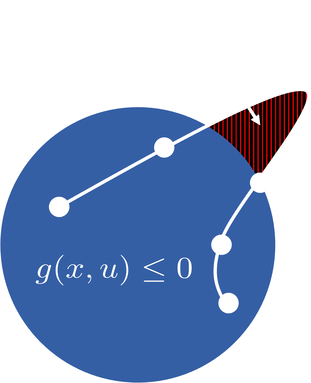
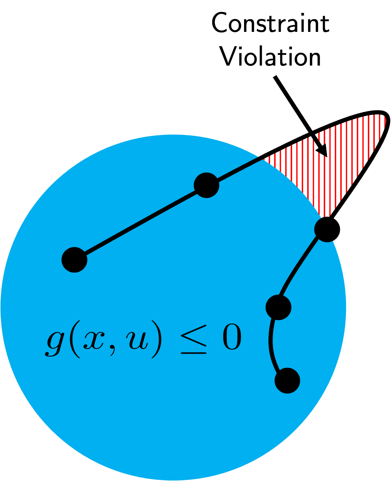
Path constraints are meant to hold for all time, but a node-based transcription only checks them at the discretization nodes — leaving the solution free to violate them between nodes. OpenSCvx closes this gap with continuous-time constraint satisfaction (CTCS): it reformulates a path constraint as an integral condition on an augmented state, so satisfying it at the nodes guarantees satisfaction throughout the interval.
The augmented penalty state
Write each path constraint in canonical form \(g(x, u) \le 0\). For a group of CTCS constraints, OpenSCvx adds one augmented state \(y\) whose derivative accumulates a non-negative penalty of the constraint violations:
where the default penalty is the squared ReLU \(\max(0, g_j)^2\) (Huber and smooth ReLU are also available, or you can write your own), and \(s\) is the time-dilation factor. Because the integrand is non-negative, \(y\) is monotonically non-decreasing and accumulates any violation occurring between nodes.
Enforcing \(y \equiv 0\) then drives every penalty — and hence every constraint — to zero continuously. In practice the convex subproblem (i) resets \(y\) to \(0\) at the start of each enforcement interval and (ii) bounds the per-segment increment,
so a small \(y_{\max}\) makes the between-node violation provably small. This is the isoperimetric-style reformulation: a bounded integral of the violation stands in for an infinite family of pointwise constraints.
Declaring CTCS constraints
Wrap any path constraint with ox.ctcs, or call .over(...) on a constraint to
restrict it to a node interval:
import openscvx as ox

constraints = [
    ox.ctcs(state <= state.max),
    ox.ctcs(state.min <= state, penalty="huber"),
    (distance >= obstacle_radius).over((0, N)),
]
Constraints sharing an enforcement interval are grouped onto one augmented state;
different intervals get separate states. The bound \(y_{\max}\) is the constraint's
licq_max (default \(10^{-4}\)); tighten it for stricter between-node enforcement.
After solving, the achieved continuous-time violation is reported as
results.ctcs_violation.
Custom penalties
The built-in penalties are selected by name — "squared_relu" (the default),
"huber", and "smooth_relu" — which fixes their shape and their internal
constants. When you want to tune those constants or shape the penalty yourself,
pass a callable instead:
# Widen Huber's quadratic region — not expressible with the string form.
ox.ctcs(altitude >= 10, penalty=lambda r: ox.Huber(ox.PositivePart(r), delta=0.5))

# Quadratic near the boundary, with a linear tail that keeps pushing far out.
ox.ctcs(
    speed <= v_max,
    penalty=lambda r: ox.Square(ox.PositivePart(r)) + 0.1 * ox.PositivePart(r),
)
The callable receives the canonicalized residual \(g_j(x, u)\) — the constraint
already rearranged into \(g_j \le 0\) form, so speed <= v_max arrives as
speed - v_max — and returns the expression to integrate. That result is summed
to a scalar, so a vector-valued residual may produce a vector-valued penalty. The
callable runs once, when the problem is built; from there its expression is
differentiated, sparsified, and cached exactly like a built-in penalty.
The body must be built from openscvx operations: ox.PositivePart, ox.Square,
ox.Huber (tunable delta), ox.SmoothReLU (tunable c), and ordinary
arithmetic on expressions. Reaching for jax.numpy instead — jnp.maximum(r, 0)
— returns an array rather than an expression and is rejected when the problem is
built: the penalty has to stay symbolic to be lowered into the augmented
dynamics.
Related reading
- Optimal Control Problem — where the CTCS reset-and-bound constraints enter the convex subproblem.
- Time Dilation — the \(s\) factor that also scales the CTCS dynamics.